Drawing on professional experience in geospatial and demographic analysis of Japanese real-estate data, this portfolio presents simplified demonstrations of the analytical methods I use. The examples apply those methods to public San Antonio data without exposing confidential information.
Each case begins with a practical question and ends with an interpretable result, a reproducible method, and an explicit boundary on use.
Case 01
Unsupervised spatial analysis
Local UMAP Explorer
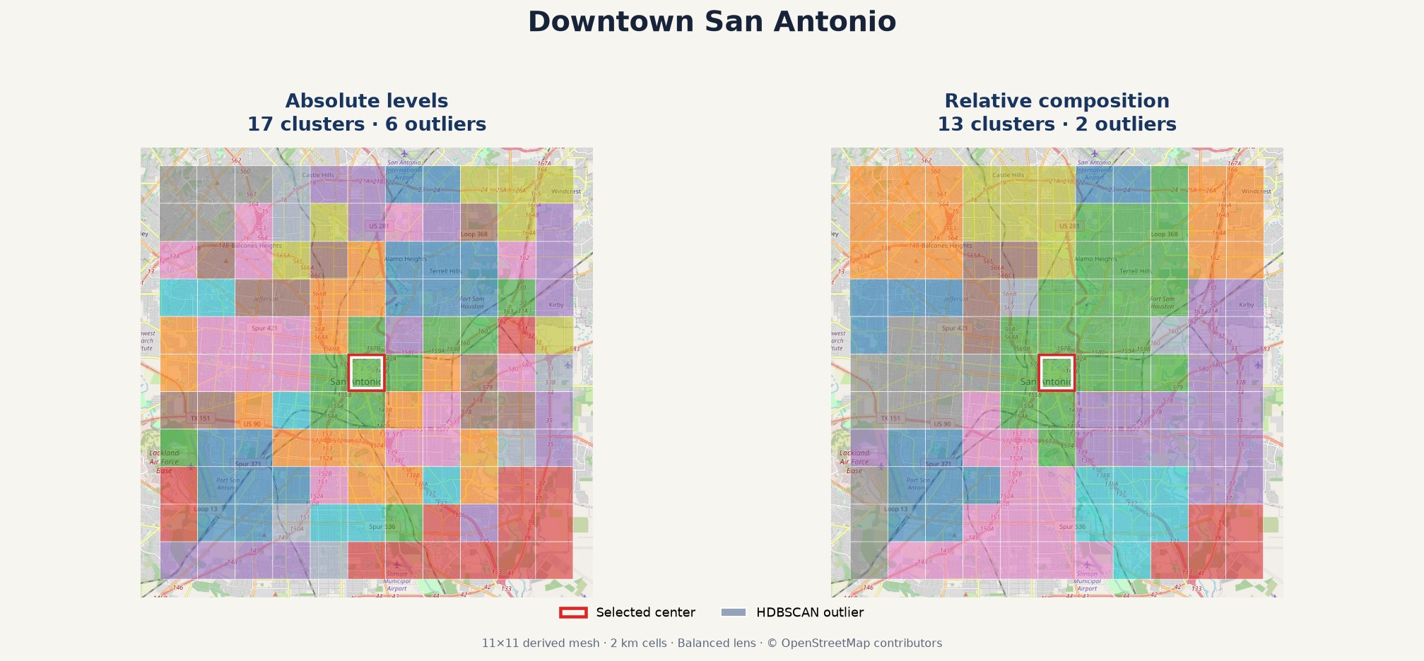
A user selects a location in San Antonio, and the tool divides the surrounding area into equal grid cells. It then compares the demographic, housing, resident-workforce, workplace-employment, and industry profile of every cell.
same color = similar profile
absolute + relative views
2 km analytical cells
Read the interpretation and method
Interpretation
The absolute view emphasizes differences in the overall scale of population and employment, while the relative view emphasizes differences in composition. Cells shown in the same color belong to the same cluster, suggesting that they have similar demographic, housing, and employment attributes. Around downtown, this separates job-intensive cells from the surrounding residential context instead of treating the entire area as one uniform center-city type.
Method
Each 2 km grid cell is described using population, income, housing, resident-worker, workplace-job, and industry variables. The variables are standardized, UMAP reduces the multivariable profiles to a lower-dimensional representation, and HDBSCAN groups cells that have similar attribute patterns.
Boundary
The colors summarize similarity in the selected data; they do not mean that two places are identical. UMAP preserves relationships among attribute profiles rather than geographic distance, and the exploratory clusters should be checked against the original variables and local knowledge.
UMAPHDBSCANmesh analysisGeoPandas
Live demonstration available on request
Complete local grid · matching colors suggest similar area profilesACS 2024 · LODES 2023 · TIGER/Line 2024
Case 02
Local site comparison
Top 10 Similar Tracts
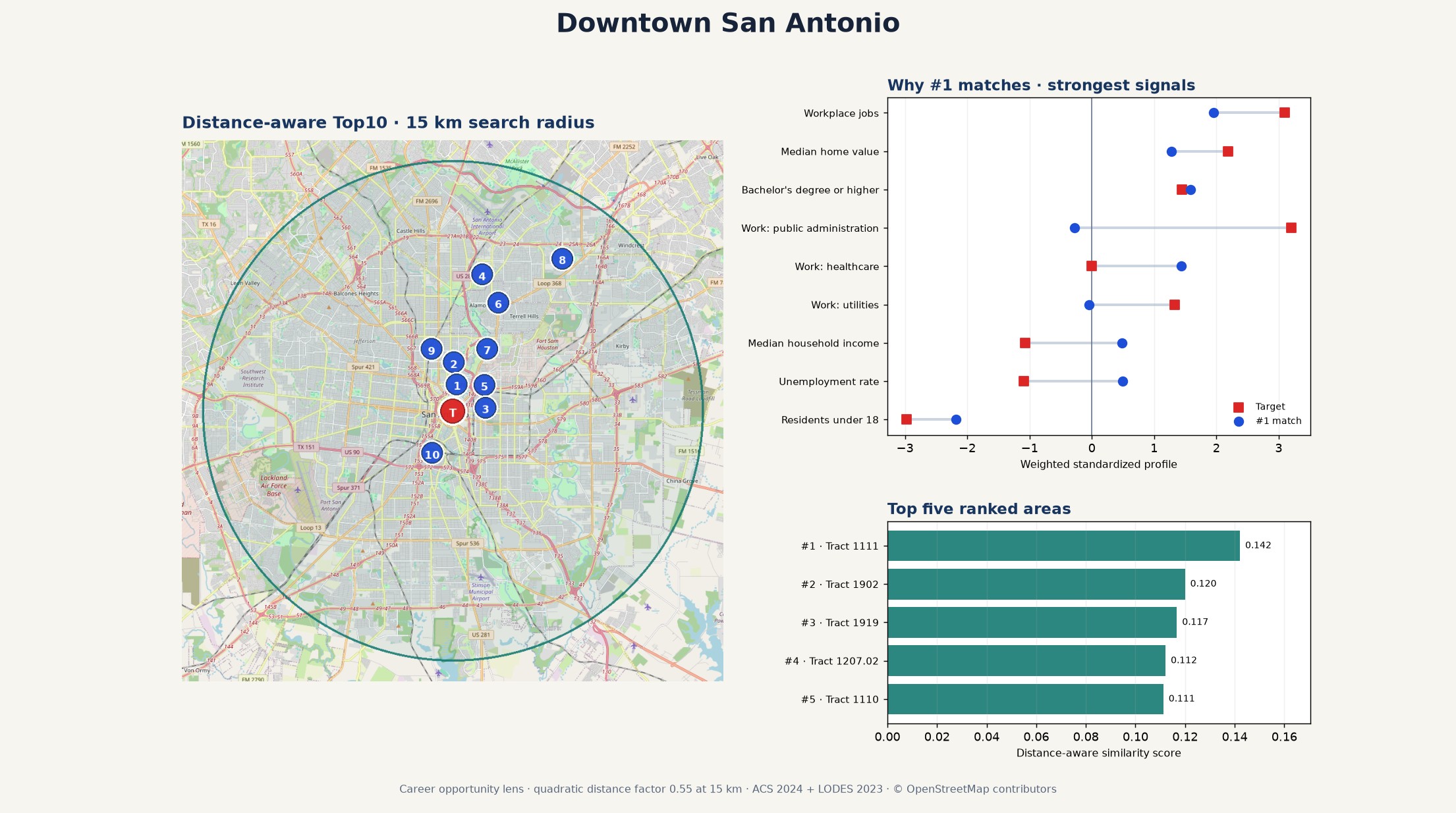
A user selects one Census tract in San Antonio. The tool compares that target with other tracts in the surrounding area and identifies the ten places whose demographic, housing, resident-workforce, and workplace-employment profiles are most similar.
one selected tract
10 ranked similar areas
optional distance adjustment
Read the interpretation and method
Interpretation
The output is a numbered map and a ranked list of ten candidate areas. A higher rank means that a tract is closer to the selected tract across the measured variables; it does not mean that the two areas are identical. When the distance-aware option is used, the score also gives preference to physically closer locations. This helps distinguish nearby alternatives from places that look similar in the data but are farther away.
Method
First, Census codes that represent missing values are removed. Highly skewed variables, such as population or job counts, are log transformed so that a few very large values do not dominate the comparison. The variables are then standardized and organized into demographic, housing, resident-workforce, and workplace-employment groups. A weighted distance calculation produces the similarity ranking, with an optional geographic-distance adjustment.
Boundary
This is an initial screening tool, not a prediction that a site is available or suitable. A highly ranked tract can still differ in land use, current vacancies, wages, travel time, employer quality, infrastructure, or parcel-level feasibility. Those factors require a separate review before making a location decision.
site selectionweighted distanceACSLODES
Live demonstration available on request
Selected target · ten ranked local matches · profile comparisonACS 2024 · LODES 2023 · TIGER/Line 2024
Case 03
Regional analogue search
Texas Top 30 Analogues
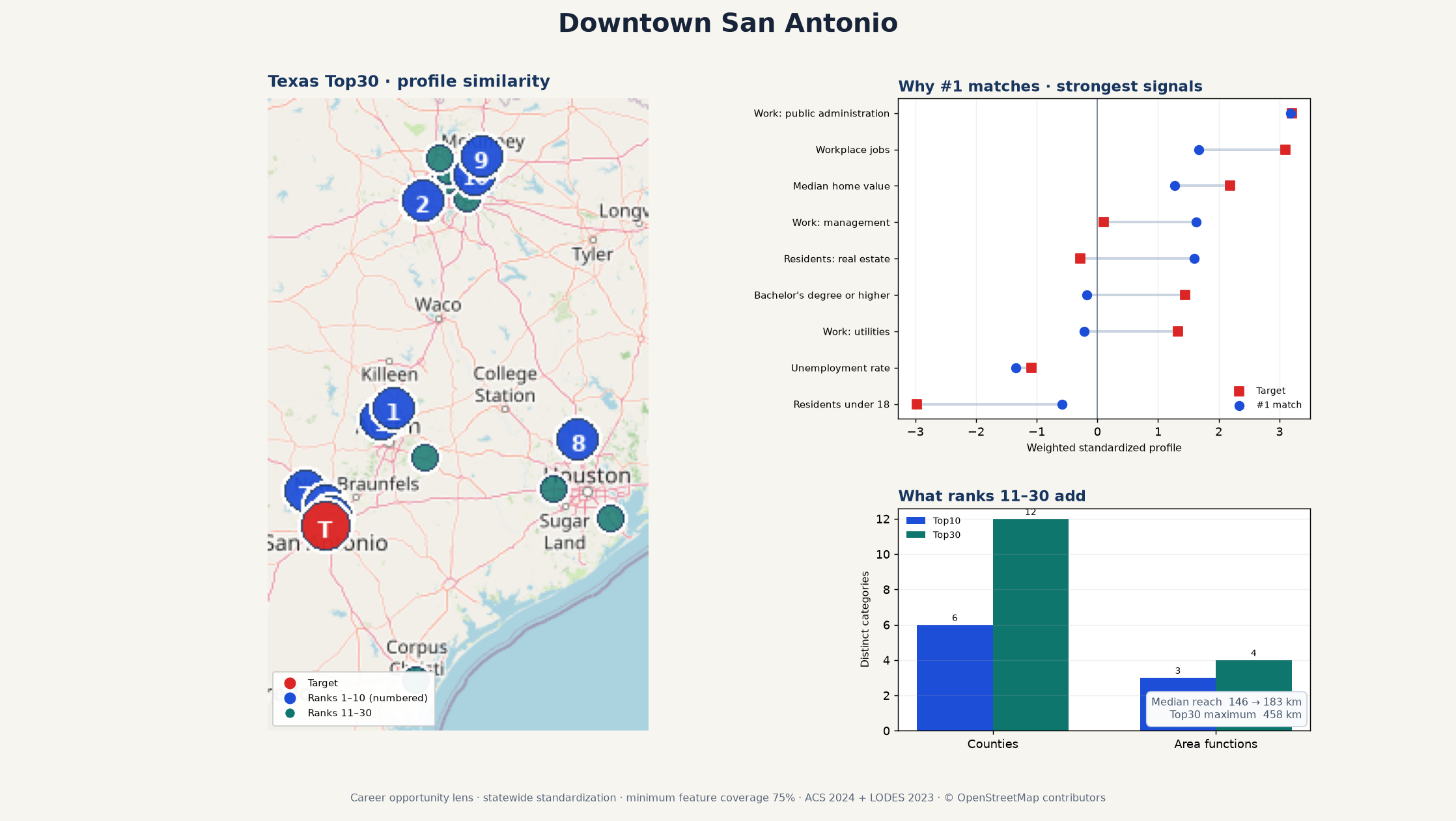
A user selects one San Antonio Census tract, and the tool searches across Texas for the thirty tracts with the most similar demographic, housing, resident-workforce, and workplace-employment profiles. The statewide search can reveal comparable areas that would be missed by looking only within the San Antonio region.
one San Antonio target
30 Texas-wide matches
county and score checks
Read the interpretation and method
Interpretation
The map shows where the thirty matches are located and whether they are concentrated near San Antonio or distributed across Texas. The ranked comparison identifies the closest statistical matches and shows which variables most strongly support the first-ranked result. County coverage and the added contribution of ranks eleven through thirty are reported so that users can judge whether the search found genuinely broader evidence or simply more matches from the same few places.
Method
The same missing-value treatment, transformation, standardization, and feature-group weighting are applied to every eligible Texas tract. The tool calculates each tract's multivariable distance from the selected San Antonio tract, sorts the results, and reports the top thirty. Diagnostics show the similarity score, geographic distribution, county representation, and the demographic, housing, and employment signals behind the ranking.
Boundary
A Texas tract can be statistically similar to the selected San Antonio tract while operating in a different policy, land-use, infrastructure, labor-market, or competitive environment. The Top30 list identifies places worth investigating; it does not establish that the locations are interchangeable or that any one of them is appropriate for a final investment or site decision.
regional analysisrankingdiagnosticsTexas
Live demonstration available on request
San Antonio target · thirty statewide matches · county coverageACS 2024 · LODES 2023 · TIGER/Line 2024
Case 04
Accessibility + spatial statistics
Job Access & Transit Equity
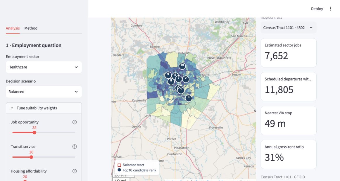
The user selects an employment sector and the tool scores each eligible Bexar County Census tract using four separate signals: estimated jobs in that sector, scheduled VIA transit service, housing affordability, and the size of the resident workforce. The map shows where those conditions reinforce one another—and where job opportunity is not matched by the other conditions.
375 Bexar County tracts
4 score components
800 m default transit buffer
How the score and spatial statistic are interpreted
What the default result says
With Healthcare, Balanced weights, and an 800 m transit buffer selected, 282 of the 375 tracts pass the data and minimum-job requirements. High-scoring tracts perform relatively well across the combined criteria; they are not necessarily the tracts with the most healthcare jobs alone. The selected downtown tract, for example, has exceptionally strong job opportunity and scheduled transit but a weaker housing-affordability component.
What Moran's I adds
Global Moran's I is approximately 0.311. Because the value is positive, tracts with similar suitability scores tend to occur near one another instead of being scattered independently across the county. A permutation pseudo-p value of 0.005 means that a pattern this strong appeared very rarely when the tract scores were randomly reassigned. This supports a county-level conclusion that accessibility is spatially clustered; it does not identify the cause of each individual cluster.
How the score is built
LODES employment estimates provide sector jobs, VIA GTFS provides scheduled weekday departures near each tract representative point, and ACS variables describe affordability and the resident workforce. Each component is converted to a 0–100 percentile relative to Bexar County and combined with visible user-controlled weights. Distance calculations use EPSG:26914. The clustering test uses shared tract boundaries (Queen contiguity) and 199 deterministic label permutations.
What the result does not claim
GTFS describes scheduled service, not observed reliability. A straight-line buffer around a representative point is not a pedestrian-network travel area. The model also omits current vacancies, wages, travel time, employer quality, and parcel-level feasibility. The output is therefore a transparent screening surface for follow-up investigation, not a final site recommendation.
GTFSEPSG:26914Moran's Isensitivity
Live demonstration available on request
Healthcare · Balanced weights · 800 m bufferDarker tract color = higher combined score
Method you can audit
From public data to a defensible decision artifact.
The portfolio emphasizes transferable GIS practice: documented assumptions, projected-coordinate operations, diagnostic outputs, and communication of uncertainty.
01Acquire
Versioned ACS, TIGER/Line, LODES, and GTFS sources with explicit vintages.
02Prepare
Sentinel handling, missing-value checks, CRS validation, transforms, and reproducible joins.
03Analyze
Similarity, clustering, proximity, accessibility, autocorrelation, and sensitivity analysis.
04Explain
Maps, profile plots, ranked diagnostics, fixed case studies, and stated limitations.
Role alignment
Built for the work behind the job title.
These projects connect Python-based geospatial analysis to the workflows used in site location, GIS production, public-sector planning, and utility data support.
Live demonstration available on request. I can walk through a selected San Antonio area, the data pipeline, analytical choices, and the limits of the result.